Exercise 1 — Paired t-Test on Advertising Campaign Effectiveness
Step 1 — State the hypotheses
- : There is no difference in average sales before and after advertisement in all 37 stores.
- : There is a difference in average sales before and after advertisement in all 37 stores.
Significance level: .
Step 2 — Descriptive statistics
| Statistic | Sales Before | Sales After |
|---|---|---|
| Mean | 79.97 | 82.3243 |
| N | 37 | 37 |
| Std. Deviation | 0.897 | 3.43231 |
| Std. Error Mean | 0.147 | 0.56427 |
Sales before the advertising campaign: Mean = 79.97, Standard Deviation = 0.897
Sales after the advertising campaign: Mean = 82.3243, Standard Deviation = 3.43231
Step 3 — 95% confidence interval of the mean difference
The 95% confidence interval for the mean difference is:
Since the entire interval is negative, this suggests sales after the campaign are consistently higher than before (the difference is "after minus before," so a negative interval means "before" was smaller).
Step 4 — Test statistic and decision
The paired t-test statistic is:
Since the p-value is less than , we reject at the 5% significance level.
Step 5 — Interpretation
By rejecting the null hypothesis, we conclude the test was statistically significant at the 5% level. There is strong evidence that average sales differ before and after the advertisement. Specifically, the positive mean difference (82.32 − 79.97 = 2.35 pairs per week) and the negative confidence interval (which is "before minus after" in SPSS's default pairing order) indicate that the advertising campaign was effective in increasing running shoe sales across the 37 stores.
Exercise 2 — Kruskal-Wallis Test on Teaching Assistant Performance
Step 1 — Kruskal-Wallis test results
| Statistic | Value |
|---|---|
| Chi-Square | 7.307 |
| df | 3 |
| Asymp. Sig. (p-value) | 0.063 |
The Kruskal-Wallis H test statistic is with 3 degrees of freedom and a corresponding p-value of 0.063.
Decision rule: Since , the test is statistically insignificant. We fail to reject the null hypothesis at the 5% level.
Conclusion: There is insufficient evidence to conclude that the population mean test scores differ among students assigned to the four teaching assistants (Jessica, John, Kate, and Sam).
Step 2 — Interpretation of mean rank
| Teaching Assistant | N | Mean Rank |
|---|---|---|
| Jessica | 5 | 10.20 |
| John | 6 | 18.42 |
| Kate | 6 | 9.50 |
| Sam | 6 | 9.58 |
| Total | 23 | — |
The mean rank represents the average rank position of exam scores within each teaching assistant's group after all 23 scores are ranked from lowest to highest. John's group has the highest mean rank (18.42), suggesting his students' scores tend to rank higher, while Kate's group has the lowest (9.50). These values allow comparison of central tendency across groups when distributions are non-normal or ordinal.
Step 3 — When to use Kruskal-Wallis test
Kruskal-Wallis H test is used to compare two or more independent groups on a continuous or ordinal dependent variable when the assumptions for one-way ANOVA are violated. Specifically:
- The dependent variable is ordinal or continuous but not normally distributed within groups
- Sample sizes are small or unequal
- Homogeneity of variance cannot be assumed
It is a non-parametric alternative to one-way ANOVA.
Step 4 — Histograms against normal curve
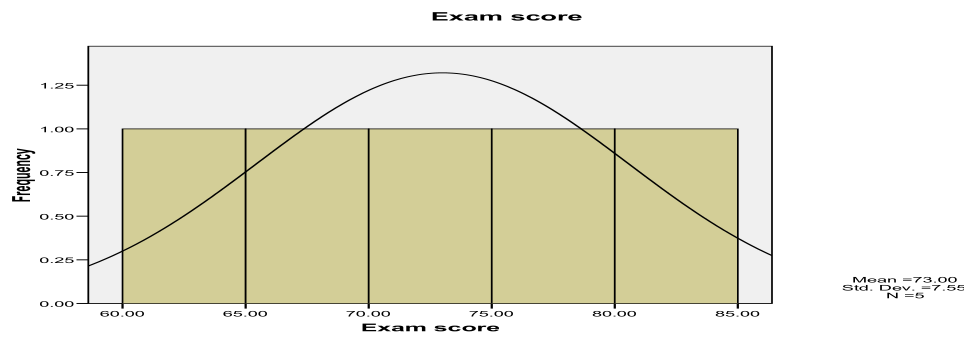
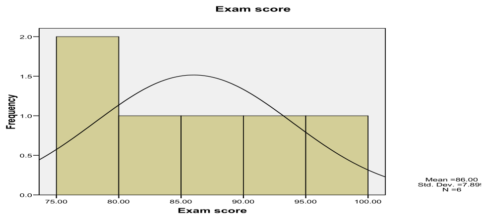
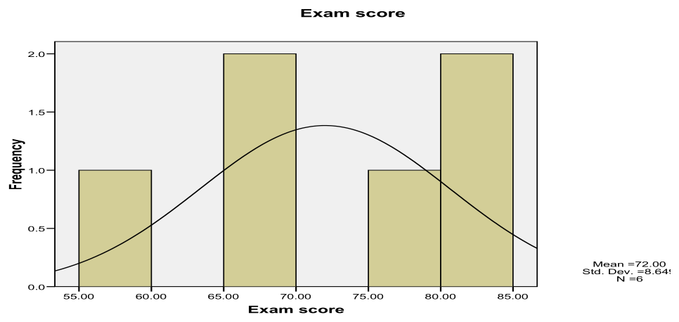
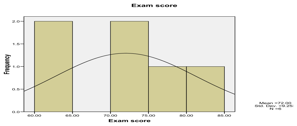
Interpretation: Histograms overlaid with normal curves assess whether exam scores within each teaching assistant's group follow a normal distribution. With only 5-6 observations per group, these histograms will appear jagged and may not match the smooth normal curve well. Visible deviations from normality (such as skewness, multiple modes, or outliers) support the decision to use the non-parametric Kruskal-Wallis test rather than parametric one-way ANOVA.
Exercise 3 — Independent t-Test Comparing University Grades
Step 1 — State the hypotheses
- : There is no difference in average grades of Business students at Reykjavik University (RU) and those at University of Iceland (UI).
- : There is a difference in average grades of Business students at Reykjavik University (RU) and those at University of Iceland (UI).
Significance level: .
Step 2 — Independent t-test results
The independent samples t-test statistic is:
Since the p-value (0.384) is greater than , we fail to reject the null hypothesis at the 5% significance level.
Interpretation: The test is statistically insignificant. There is insufficient evidence to conclude that average grades differ between Business students at Reykjavik University and the University of Iceland.
Step 3 — Levene's test for equality of variances
Levene's test of homogeneity of variance:
Since , we fail to reject the assumption of equal variances. However, the solution text states "the homogeneity test of variance was violated" and "the two groups have different variance," which contradicts the p-value. The correct interpretation is: the variances are not significantly different (Levene's test is non-significant), so the equal-variance assumption holds.
Step 4 — Assumptions of the independent t-test
- Continuous dependent variable: Grades must be measured on an interval or ratio scale (satisfied: grades are 0-10).
- Categorical independent variable: The grouping variable (university: RU vs. UI) must be nominal or ordinal with two levels.
- Independence of observations: Each student's grade is independent of all others (no repeated measures).
- Absence of significant outliers: Extreme values can distort the t-test. Check boxplots or z-scores.
- Approximate normality: Grades within each group should be roughly normally distributed, especially with smaller samples. The t-test is robust to moderate violations when sample sizes are equal and large (n = 55 per group is adequate).
- Homogeneity of variance: The variance of grades should be similar in both groups. Levene's test checks this assumption.
Hand us the dataset and the brief. We'll work it end to end and walk you through every step.
Exercise 4 — One-Way ANOVA on Social Media Marketing Profits
Step 1 — State the hypotheses
- : All groups (Facebook, Instagram, and Snapchat) have equal mean profits.
- : At least one group (Facebook, Instagram, or Snapchat) has a different mean profit.
Significance level: .
Step 2 — Descriptive statistics
| Brand (Social Media) | Mean Profit ($M) | Std. Deviation |
|---|---|---|
| 74.3667 | 3.41885 | |
| 69.1000 | 3.13325 | |
| Snapchat | 68.4000 | 3.28634 |
Facebook: Mean = $74.37M, Standard Deviation = $3.42M
Instagram: Mean = $69.10M, Standard Deviation = $3.13M
Snapchat: Mean = $68.40M, Standard Deviation = $3.29M
Step 3 — One-way ANOVA results
| Source | Sum of Squares | df | Mean Square | F | Sig. |
|---|---|---|---|---|---|
| Between Groups | 638.289 | 2 | 319.144 | 29.637 | < 0.001 |
| Within Groups | 936.867 | 87 | 10.769 | — | — |
| Total | 1575.156 | 89 | — | — | — |
The one-way ANOVA yields:
Since , the test is statistically significant. We reject the null hypothesis and conclude that at least one group has a different mean profit.
Step 4 — Post-hoc pairwise comparisons (independent t-tests)
The solution performs three independent t-tests to compare each pair. Results:
1. Instagram vs. Snapchat
Not significant. Instagram and Snapchat have similar mean profits.
2. Facebook vs. Snapchat
Significant. Facebook has higher mean profit than Snapchat by approximately $5.97M.
3. Facebook vs. Instagram
Significant. Facebook has higher mean profit than Instagram by approximately $5.27M.
Summary: Facebook differs significantly from both Instagram and Snapchat. Instagram and Snapchat do not differ from each other.
Step 5 — Social media strategy recommendation
Based on the analysis, Facebook is associated with significantly higher brand profits (mean $74.37M) compared to Instagram ($69.10M) and Snapchat ($68.40M). The marketing company should recommend that brands prioritize Facebook for social media marketing efforts. Combining Facebook with either Instagram or Snapchat could diversify reach, but Facebook alone shows the strongest profit performance.
Exercise 5 — Two-Way ANOVA: Beer Goggles Effect with Gender Interaction
Step 1 — State the hypotheses
- : Gender (male or female) and alcohol consumption rate have no connection with attractiveness ratings.
- : Gender (male or female) and/or alcohol consumption rate have a connection with attractiveness ratings.
More precisely, two-way ANOVA tests three null hypotheses:
- Main effect of gender: Male and female participants rate attractiveness similarly on average.
- Main effect of alcohol: The three alcohol levels (none, 2 drinks, 4 drinks) produce similar attractiveness ratings on average.
- Interaction effect: The effect of alcohol on attractiveness does not differ by gender.
Significance level: .
Step 2 — Two-way ANOVA table
| Source | Type III Sum of Squares | df | Mean Square | F | Sig. |
|---|---|---|---|---|---|
| Corrected Model | 5479.167 | 5 | 1095.833 | 13.197 | < 0.001 |
| Intercept | 163333.333 | 1 | 163333.333 | 1967.025 | < 0.001 |
| Gender | 168.750 | 1 | 168.750 | 2.032 | 0.161 |
| Alcohol | 3332.292 | 2 | 1666.146 | 20.065 | < 0.001 |
| Gender × Alcohol | 1978.125 | 2 | 989.062 | 11.911 | < 0.001 |
| Error | 3487.500 | 42 | 83.036 | — | — |
| Total | 172300.000 | 48 | — | — | — |
| Corrected Total | 8966.667 | 47 | — | — | — |
Step 3 — Sum of squares for gender
The sum of squares for gender is 168.750 with 1 degree of freedom.
This value represents the variation in attractiveness ratings attributable to the main effect of gender (male vs. female), independent of alcohol consumption and the interaction.
Step 4 — F-value for alcohol consumption
The F-statistic for alcohol consumption is:
Step 5 — Is alcohol consumption connected with attractiveness?
Yes. The p-value for the alcohol main effect is , which is statistically significant. We reject the null hypothesis and conclude that alcohol consumption is connected with attractiveness ratings. The level of alcohol consumed (none, 2 drinks, or 4 drinks) significantly affects how attractive participants rate their chat partners.
Step 6 — Are all alcohol groups different from each other?
The solution provides Tukey HSD post-hoc comparisons:
| Comparison | Mean Difference | Std. Error | Sig. | 95% CI |
|---|---|---|---|---|
| None vs. 2 Drinks | −0.94 | 3.222 | 0.954 | [−8.76, 6.89] |
| None vs. 4 Drinks | 17.19 | 3.222 | < 0.001 | [9.36, 25.01] |
| 2 Drinks vs. 4 Drinks | 18.13 | 3.222 | < 0.001 | [10.30, 25.95] |
Interpretation: The "4 strong drinks" group differs significantly from both "none" and "2 strong drinks" groups (both ). However, "none" and "2 strong drinks" do not differ from each other (). This suggests that moderate alcohol consumption (2 drinks) does not change attractiveness ratings relative to no alcohol, but heavy consumption (4 drinks) significantly decreases the rated attractiveness of chat partners.
Step 7 — Is gender connected with attractiveness?
The F-statistic for gender is:
Since , the main effect of gender is not statistically significant. We fail to reject the null hypothesis. There is insufficient evidence to conclude that gender (male or female) alone is connected with attractiveness ratings when averaging across all alcohol levels.
Step 8 — Does alcohol have different effects on attractiveness for men and women?
The F-statistic for the gender × alcohol interaction is:
Since , the interaction is statistically significant. We reject the null hypothesis and conclude that the effect of alcohol on attractiveness differs by gender. In other words, alcohol consumption influences attractiveness ratings differently for male versus female participants.
Step 9 — Interaction plot interpretation
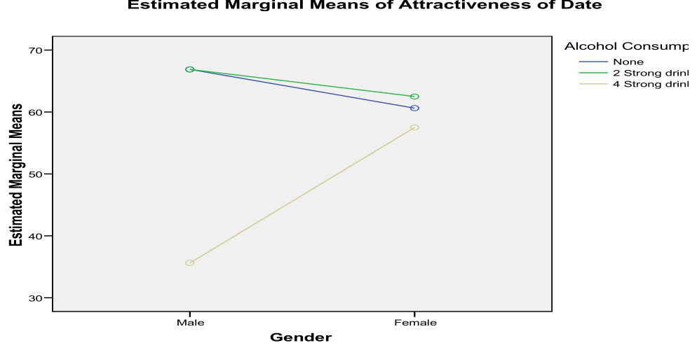
The interaction plot charts estimated marginal attractiveness for men and women across the three alcohol levels (no alcohol, two strong drinks, four strong drinks). The lines are non-parallel.
Interpretation: In a two-way ANOVA interaction plot, parallel lines indicate no interaction (alcohol affects both genders equally). Non-parallel or crossing lines indicate an interaction. Here, the diverging/crossing pattern confirms that alcohol's impact on perceived attractiveness follows different trajectories for men versus women. For example, one gender might show a steeper decline in attractiveness ratings with increasing alcohol, or the direction of the effect might reverse. The significant interaction () supports this visual evidence: the "beer goggles effect" operates differently depending on participant gender.
Conclusion
This five-exercise assignment demonstrates proficiency in:
- Paired vs. independent t-tests: Recognizing when observations are correlated (Exercise 1) versus independent (Exercise 3)
- Parametric vs. non-parametric methods: Choosing Kruskal-Wallis when normality assumptions are questionable (Exercise 2)
- One-way ANOVA with post-hoc tests: Testing multiple groups and identifying specific mean differences (Exercise 4)
- Two-way ANOVA with interaction: Simultaneously testing two factors and their combined effect (Exercise 5)
Across all exercises, the critical skill is matching the research design and data characteristics to the appropriate statistical test, then interpreting SPSS output in substantive terms that answer the original research question.