Introduction
This assignment evaluates descriptive statistics, confidence interval estimates, correlation analysis, and simple linear regression using SPSS. The data is analyzed at two levels: the full population (N = 32 NFL teams) and a random sample (n = 11 teams). The two variables examined are Current Value (in millions of dollars) and Operating Income (in millions of dollars). Both variables are numerical with a scale level of measurement.
Part 1 — Descriptive Statistics of the Population (N = 32)
Descriptive Statistics Table
| N | Sum | Mean | Std. Deviation | Median | Skewness | Kurtosis | |
|---|---|---|---|---|---|---|---|
| Current Value (in Millions $) | 32 | 62910 | 1965.94 | 629.418 | 1760 | 1.505 | 2.164 |
| Operating Income (in Millions $) | 32 | 2438.8 | 76.212 | 50.4451 | 61.550 | 2.326 | 6.676 |
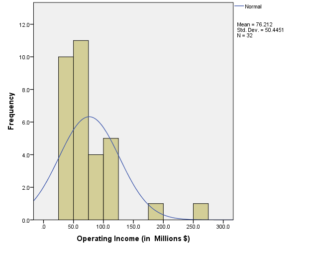
Discussion: The population (N = 32) shows a mean current value of $1965.94 million with a standard deviation of $629.418 million, and a median of $1760 million. Operating income has a mean of $76.212 million, standard deviation of $50.4451 million, and median of $61.550 million. Both variables show positive skewness (1.505 and 2.326 respectively), indicating right-skewed distributions with a long tail of high-value teams.
Histograms
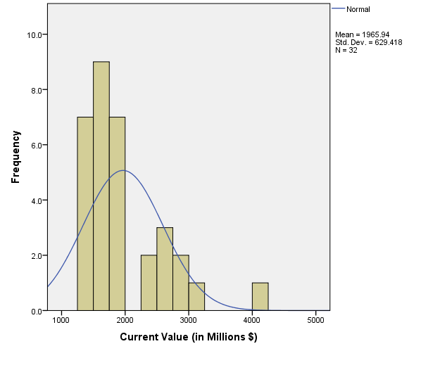
Discussion: The population (N = 32) histograms for Current Value and Operating Income show that the scores do not have a normal distribution (no perfect bell-shaped curve) — the graphs are skewed to the right. This indicates that most teams have moderate valuations and incomes, with a few high-revenue franchises pulling the mean above the median.
Part 2 — Random Sample Selection and Descriptive Statistics (n = 11)
Simple Random Sample (n = 11)
| 2015 Rank | Team | Current Value (in Millions $) | Operating Income (in Millions $) |
|---|---|---|---|
| #28 | St Louis Rams | 1450 | 34.00 |
| #23 | New Orleans Saints | 1520 | 70.00 |
| #12 | Baltimore Ravens | 1930 | 59.80 |
| #26 | Tennessee Titans | 1490 | 50.50 |
| #19 | Carolina Panthers | 1560 | 77.80 |
| #22 | San Diego Chargers | 1530 | 64.80 |
| #14 | Indianapolis Colts | 1880 | 90.10 |
| #30 | Detroit Lions | 1440 | 36.10 |
| #21 | Kansas City Chiefs | 1530 | 48.60 |
| #15 | Seattle Seahawks | 1870 | 43.60 |
| #3 | Washington Redskins | 2850 | 124.90 |
Descriptive Statistics Table (Sample)
| N | Sum | Mean | Std. Deviation | Median | Skewness | Kurtosis | |
|---|---|---|---|---|---|---|---|
| Current Value (in Millions $) | 11 | 19050 | 1731.82 | 413.469 | 1530 | 2.281 | 5.800 |
| Operating Income (in Millions $) | 11 | 700.2 | 63.655 | 26.7346 | 59.800 | 1.219 | 1.645 |
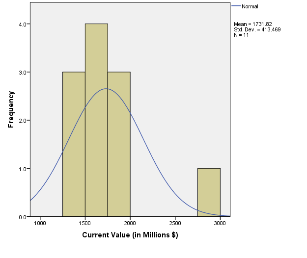
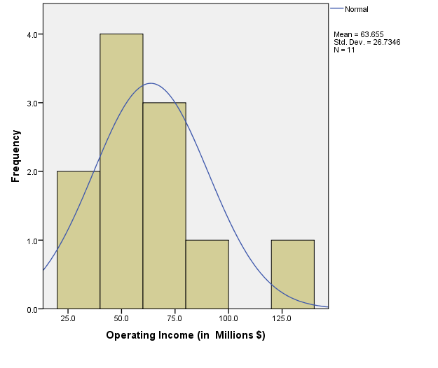
Discussion: The sample (n = 11) shows a mean current value of $1731.82 million with a standard deviation of $413.469 million and a median of $1530 million. Operating income has a mean of $63.655 million, standard deviation of $26.7346 million, and median of $59.800 million. The standard deviations are notably smaller than the population values, reflecting reduced variability in this particular sample.
Histograms (Sample)
Discussion: The sample size (n = 11) histograms for Current Value and Operating Income show that the scores are approximately normally distributed (reasonably well-shaped bell curves). This is expected for small samples drawn from skewed populations — individual samples may appear more symmetric than the parent distribution.
Part 3 — Comparison of Population and Sample
Comparison Table
| Current Value ($M) | Operating Income ($M) | |
|---|---|---|
| Population Mean | 1965.94 | 76.212 |
| Population Std. Deviation | 629.418 | 50.4451 |
| Population Median | 1760 | 61.550 |
| Sample Mean | 1731.82 | 63.655 |
| Sample Std. Deviation | 413.469 | 26.7346 |
| Sample Median | 1530 | 59.800 |
Discussion: The mean, standard deviation, and median of the population (N = 32) are observed to be higher than the corresponding sample (n = 11) statistics for both Current Value and Operating Income. The differences are substantial: the population mean for Current Value is $234.12 million higher than the sample mean, and the population standard deviation is $215.95 million higher. This reflects sampling variability — this particular random sample happened to exclude some of the highest-valued teams (e.g., Dallas Cowboys, New England Patriots) that pull the population mean upward.
Part 4 — Confidence Interval Estimates (95% Level)
Current Value ($M)
Sample mean:
Sample standard deviation:
Sample size:
Standard error:
For a 95% confidence interval, using :
Discussion: The 95% confidence interval for Current Value is million. The population mean of $1965.94 million is contained within this interval, meaning our sample-based estimate successfully captures the true population parameter.
Operating Income ($M)
Sample mean:
Sample standard deviation:
Sample size:
Standard error:
For a 95% confidence interval:
Discussion: The 95% confidence interval for Operating Income is million. The population mean of $76.212 million is contained within this interval, confirming that our sample provides a reliable estimate of the population parameter.
Hand us the dataset and the brief. We'll work it end to end and walk you through every step.
Part 5 — Correlation Analysis
Population (N = 32)
Pearson Correlation:
Significance: (two-tailed)
Discussion: A very strong and statistically significant positive correlation () is observed between Current Value and Operating Income across the population of N = 32 teams. The p-value is less than 0.001, indicating that this relationship is highly unlikely to have occurred by chance. Teams with higher operating incomes tend to have substantially higher current valuations.
Sample (n = 11)
Pearson Correlation:
Significance: (two-tailed)
Discussion: A strong and statistically significant positive correlation () is observed between Current Value and Operating Income in the sample of n = 11 teams. The p-value of 0.004 is well below the conventional 0.05 threshold, confirming that the relationship remains significant even in the smaller sample. The sample correlation is somewhat lower than the population correlation (0.791 vs. 0.918), which is typical of sampling variability.
Part 6 — Simple Linear Regression Analysis (Sample, n = 11)
Model Specification and Features
Model Summary:
| R | R² | Adjusted R² | Std. Error of the Estimate |
|---|---|---|---|
| 0.791 | 0.626 | 0.585 | 266.435 |
Coefficients:
| Term | B | Std. Error | t | Sig. |
|---|---|---|---|---|
| (Constant) | 952.734 | 216.094 | 4.409 | 0.002 |
| Operating Income | 12.239 | 3.151 | 3.884 | 0.004 |
Features: The coefficient of determination () is 0.626, meaning that 62.6% of the variability in Current Value is explained by Operating Income. Both the constant (intercept) and slope coefficients are statistically significant (p = 0.002 and p = 0.004 respectively), indicating that the regression model is meaningful.
Variables
Independent variable (X): Operating Income (in millions of dollars)
Dependent variable (Y): Current Value (in millions of dollars)
Regression Equation
where is the predicted Current Value and Operating Income is measured in millions of dollars.
Regression Line and Scatter Plot
Discussion: The scatter plot shows a clear positive linear relationship between Operating Income and Current Value. The regression line fits the data reasonably well, with most points clustered around the line. The Washington Redskins (Operating Income = $124.9M, Current Value = $2850M) appears as a high-leverage point in the upper right.
Residuals
Discussion: Residuals represent the vertical distances between the observed Current Value and the predicted value from the regression line. Positive residuals indicate teams valued higher than the model predicts; negative residuals indicate teams valued lower than predicted. The residual plot helps diagnose whether the linear model is appropriate and whether assumptions like constant variance are met.
Interpretation of Coefficients
Intercept (): When Operating Income is zero, the model predicts a Current Value of $952.734 million. This represents the baseline value of an NFL franchise independent of operating income, though extrapolating to zero income is beyond the range of the data and may not be meaningful.
Slope (): For each additional $1 million in Operating Income, the model predicts an increase of $12.239 million in Current Value. This is a substantial multiplier effect — profitability strongly drives franchise valuation in the NFL market.
Forecasting Y for Three X Values
Using the regression equation :
| Operating Income (X) | Calculation | Predicted Current Value (Y) |
|---|---|---|
| $54 | $952.734 + 12.239(54) = 952.734 + 660.906$ | $1613.64 |
| $67.70 | $952.734 + 12.239(67.70) = 952.734 + 828.580$ | $1781.31 |
| $93 | $952.734 + 12.239(93) = 952.734 + 1138.227$ | $2090.96 |
Forecasted values:
- million
- million
- million
All three X values fall within the range of the sample data (min = $34.00M, max = $124.90M), so these predictions are reasonable interpolations rather than risky extrapolations.
Part 7 — Conclusion
In the descriptive comparison, the mean, standard deviation, and median values for both Current Value and Operating Income were higher in the population (N = 32) than in the sample (n = 11), reflecting sampling variability and the exclusion of some high-valued franchises from this particular sample.
Both 95% confidence intervals constructed from the sample statistics successfully contained the true population means, demonstrating that the sample (despite being smaller and having lower means) provided reliable estimates of the population parameters.
The correlation analysis revealed a very strong positive relationship between Current Value and Operating Income in the population () and a strong relationship in the sample (). Both correlations were statistically significant, confirming that profitability is a key driver of franchise value.
The simple linear regression model based on the sample () explained 62.6% of the variance in Current Value. The slope coefficient of 12.239 indicates that each additional million dollars in operating income predicts a $12.239 million increase in team valuation — a powerful multiplier effect. Both the intercept and slope were statistically significant (p = 0.002 and p = 0.004 respectively), confirming the model's validity.
Forecasts for three operating income values ($54M, $67.70M, and $93M) produced current value predictions of $1613.64M, $1781.31M, and $2090.96M respectively, all within plausible ranges given the sample data. The regression model provides a useful tool for estimating NFL franchise valuations based on profitability, though the unexplained 37.4% of variance suggests other factors (market size, stadium revenue, brand strength) also play important roles.